Part 1: TUTORIAL: Creating a Classified Map Using Keras and Tensorflow

In my research with Victor Gutierrez-Velez in the Remote Sensing and Sustainability Lab at Temple University, this project involved investigating the applicability of Deep Learning and Neural Networks for automatically classifying high-resolution multi-spectral remote sensing imagery of wetlands in Colombia. This work was performed as part of my capstone project as a culmination of a Professional Science Master’s in GIS from the Department of Geography and Urban Studies at Temple University.

This post contains Part 1 of the report, and will walk through building a model using Python, Keras, and Tensorflow, and creating a classified map using code created by github user reachsumit.

Part 2 details our process customizing this code to classify imagery of the Colombian wetlands obtained from Planet Labs.

Tutorial

Preparing the Python Environment

We will install Python and all necessary tools through the Miniconda Package Manager. This creates a self-contained virtual environment where packages can be installed and upgraded without causing compatibility issues with things like ArcGIS, QGIS, and the operating system.

Conda and pip are both package managers that can install and update python packages. In this tutorial, we are using conda. Using conda and pip side by side to manage python modules is not recommended, so future packages installed in this environment should also be installed with conda.

To begin, we will download the Miniconda Python 3.7 64-bit installer. This document will focus on Windows 10, although all of the tools are cross platform, so it should also apply to MacOS and Linux.

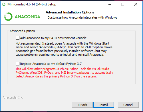
Running the installer, most of the default options should be fine. When you get to the Advanced Installation Options screen, it is important that you uncheck the option to “Register Anaconda as my default Python 3.7”. This can interfere with other software, and will not be necessary for our analysis.

Adding Anaconda to your PATH is not necessary, because it will install an Anaconda Prompt utility in your start menu that will provide a preconfigured shell in the Anaconda environment. Electing to check this option will most likely not cause problems, if you would prefer to access the conda binary from any windows shell.

After the install is complete, run the “Anaconda Prompt” utility from the start menu. To create a new Anaconda environment with Python 3.6, run the following command, and type y when prompted:
conda create --name keras python=3.6

To activate our new environment, run the following command:
conda activate keras

This next command downloads and installs a number of packages, so this may take a few minutes depending on your internet speed:
conda install spyder numpy pandas matplotlib tensorflow-mkl keras

• spyder: a Python IDE
• numpy: a package providing powerful functions for working with arrays of numbers
• pandas: provides python with dataframes similar to those in R
• matplotlib: graphing and visualization tools
• tensorflow-mkl: this is a build of tensorflow optimized for intel CPUs
• keras: the high-level API with which our scripts will interface

We also need to install the tifffile package from a different installation channel. This is the package that imports rasters and stores them as numpy arrays:
conda install -c conda-forge tifffile

Obtaining the scripts and data

For this tutorial, we will use scripts and data provided by user reachsumit on github [2]. Please download and unzip this zip file from the repository:

In Downloads\deep-unet-for-satellite-image-segmentation-master\data, you find the tiff images and corresponding masks serving as training data. The mband directory contains 24 satellite images and test.tif, an image provided without a corresponding mask that can be used to run predictions using our generated model. The gt_mband directory contains 24 stacked mask files, each one containing 5 masks outlining the shapes of buildings, roads, trees, crops, and water.

Training the Model

In the Anaconda folder in the start menu, you will find an item labeled Spyder(keras). Please run this program. This will open the Spyder Python IDE. In the file menu choose Open, navigate to the deep-unet-for-satellite-image-segmentation-master directory, and open train_unet.py.

In the course of its algorithm, this script will by default loop through the data 150 times, or epochs using tensorflow’s terminology. This is a good value to help maximize accuracy, but can take a very long time, probably a day or two depending on the machine..

For testing or debugging purposes, a much shorter run is often necessary. While we’re getting accustomed to this script, it’s recommended to set this value to something much smaller, like 10. Once we get a result we’re comfortable with, we can rename the existing model file, and re-create the model with a much higher number of epochs, which should increase accuracy significantly.

To alter the number of epochs, change the value below, found on line 23.

N_EPOCHS = 150

Using a method called data augmentation, this script by default assembles 4000 small tiles from the 24 image/mask pairs for training, and 1000 for validation of model accuracy. These two numbers, found on lines 27-28 can also be altered to decrease training time at the expense of accuracy. VAL_SIZE should be 25% of TRAIN_SIZE.

TRAIN_SZ = 4000  # train size
VAL_SZ = 1000    # validation size

By default, this script loads image tiles in groups of 150. This value affects ram used by the model, so this number can be reduced, should the script begin to cause memory problems. This value is found on line 26.

BATCH_SIZE = 150

From the Run menu, choose Run to begin training our model. The script will print status updates for our run in the Python Console in the bottom right corner.

When our run completes, it saves the model to a file at the below path, overwriting any previous model with that specific filename. Because of this behavior, it is best to make a backup copy of this file when training is complete, in the event it is accidentally overwritten by a future training run.
Model Path: deep-unet-for-satellite-image-segmentation-master\weights\unet_weights.hdf5

It will also create line graphs of Loss and Accuracy for each epoch. For further optimization of the model, the loss graph can be used to tune the number of epochs to the point with lowest loss. In addition to wasting resources, continuing past this point can be a source of overfitting in our model.
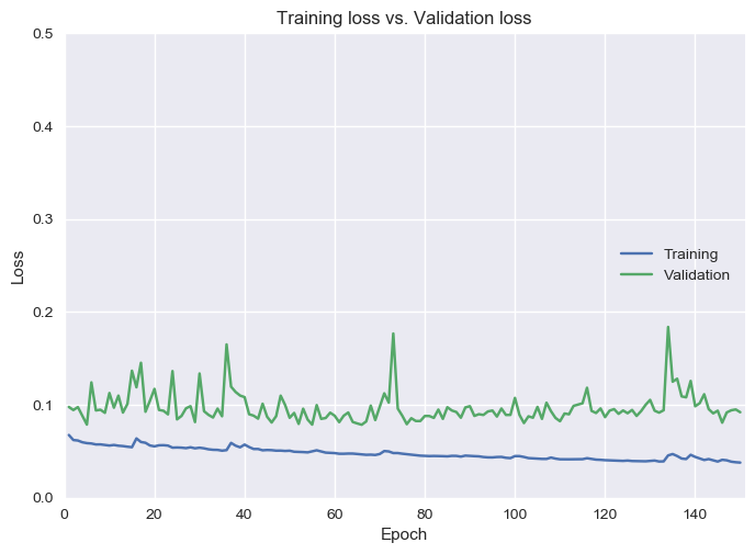loss.png

Predicting Against the Model

Now that our training run has completed and we have a model in the weights directory named unet_weights.hdf5, we can use it to create a classified map of the test image, test.tif.

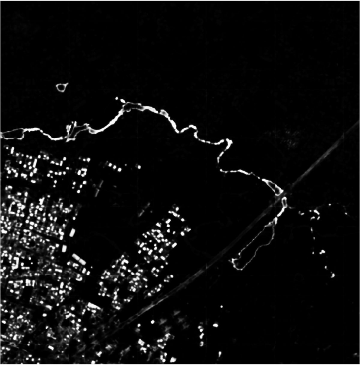
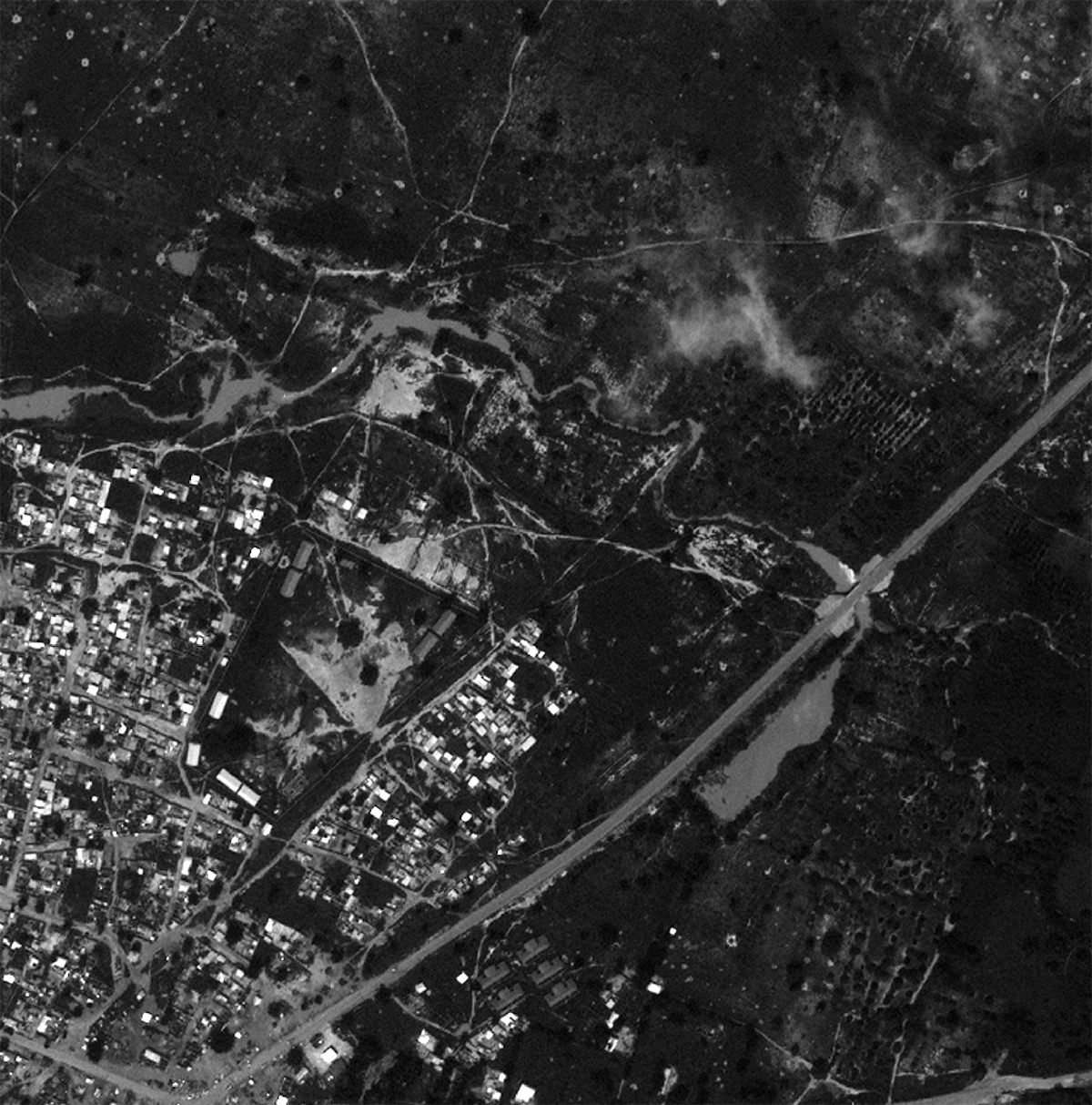test.tif

In the file menu choose Open, navigate to our deep-unet-for-satellite-image-segmentation-master directory, and open predict.py.

We will now use predictions from our model to create a classified map for our test image. The image from which to create predictions is defined in line 73.

test_id = 'test'

From the Run menu, choose Run to begin creating predictions. This will finish relatively quickly, most likely under an hour depending on the hardware.

When it completes, it will create two rasters: result.tif and map.tif. result.tif is the direct prediction created by our model, and the picture_from_mask() function reclassifies that raster based on pre-defined classes and colors. Should you wish to customize these colors, they are defined in lines 48-53.

colors = {
0: [150, 150, 150],  # Buildings
1: [223, 194, 125],  # Roads & Tracks
2: [27, 120, 55],    # Trees
3: [166, 219, 160],  # Crops
4: [116, 173, 209]   # Water

result.tif

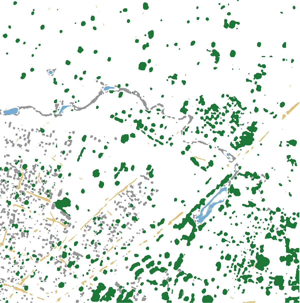
map.tif

map.tiff can now be combined with test.tif in a program like qgis or photoshop to create a classified map based on our test image. Values such as number of epochs, training size, and validation size can now be tweaked for further attempts to decrease our model’s loss.

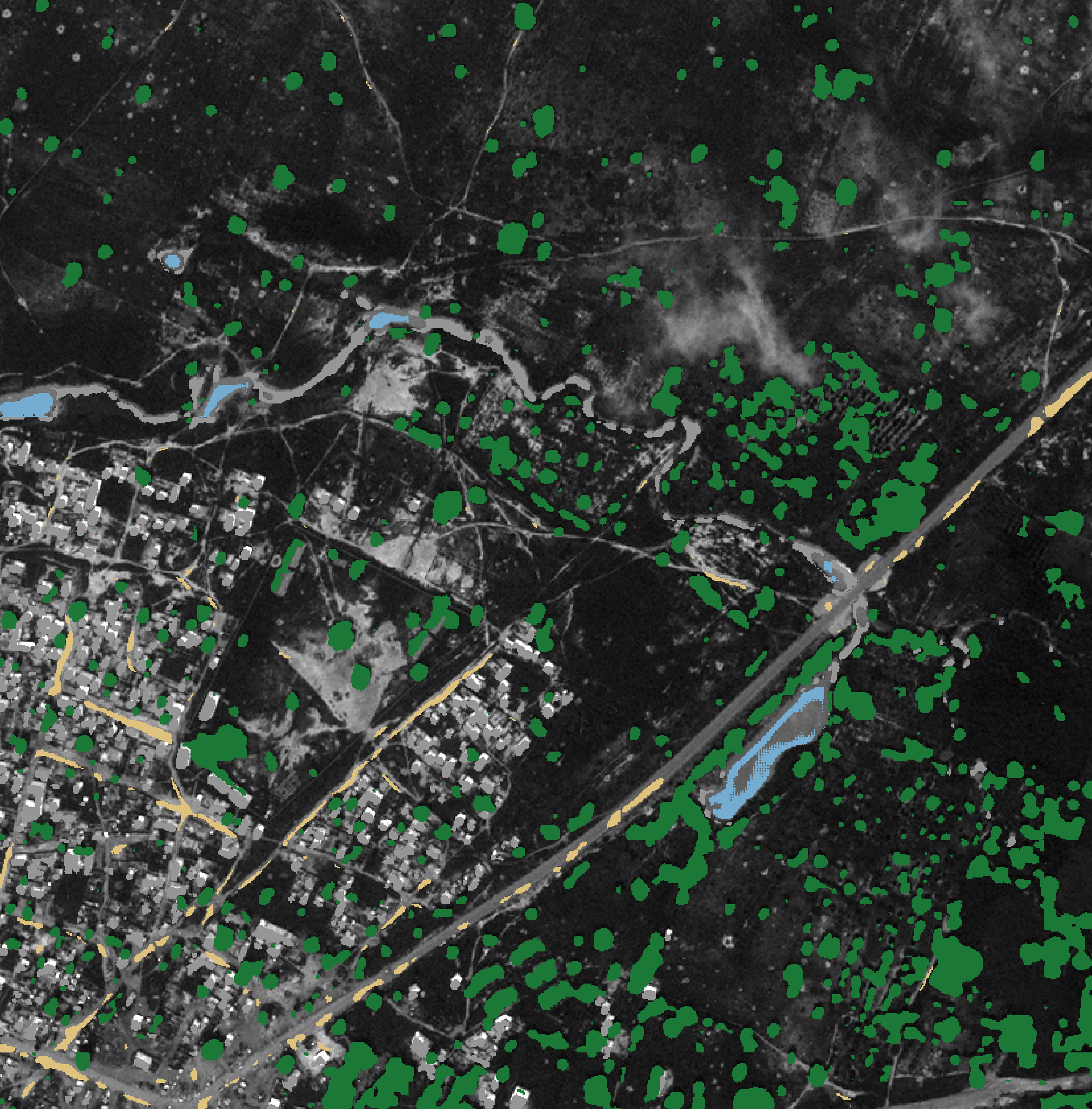
The Finished Product

Customizing the model

Report continues in Part 2