Analyzing Spatial Dependency Patterns Around Narcotics Arrests

This analysis will use spatial statistical analysis techniques in R to investigate possible correlated data, and the extent to which observed clustering is statistically significant.

Research Question

Philadelphia’s community of Heroin users and dealers is one of the tougher safety and public health issues this city has dealt with in recent memory. As we saw in a previous analysis, drug sales and communities of homeless users seem to cluster around transit infrastructure such as the Market-Frankford El, and railroad infrastructure used by freight companies. Is there a statistically significant correlation between these arrests and demography data from the 2016 American Community Survey?

Data

Dependent Variable

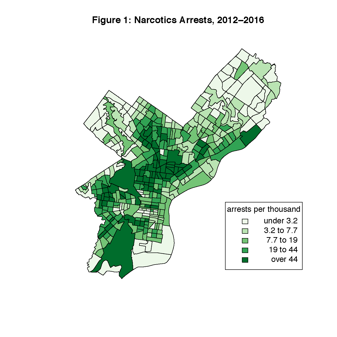
narcnorm2: narcotics arrests per 1000 people in Philadelphia between 2012 and 2016, aggregated at the census tract level. This data was originally taken from a large crime incidents dataset from Open Data Philly. Figure 1 is a map of this data by census tract. Upon visual inspection, some clustering is apparent, especially through the North Philly and Kensington areas, although it remains to be seen whether or not this is statistically significant autocorrelation.

Independent Variables

vetnorm: the rate of veterans 18 and over in the Civilian population. This has been normalized by the 18 and over civilian population. This data is from the 2016 American Community Survey 5 year estimate.

incomefix: the Per Capita income in 2016 inflation adjusted dollars. This data is from the 2016 American Community Survey 5 year estimate.

servnorm: Civilian 16 years and over employed in a service job. This has been normalized by the 16 and over civilian population. This data is from the 2016 2016 American Community Survey 5 year estimate.

             narcnorm2    vetnorm      incomefix    servnorm
min          0.000000e+00 0.000000e+00 0.000000e+00 0.000000e+00
max          1.175000e+04 1.000000e+00 9.781900e+04 1.000000e+00
median       1.253307e+01 5.128688e-02 2.038450e+04 2.456737e-01
mean         6.110455e+01 5.500923e-02 2.489282e+04 2.427069e-01
var          3.613627e+05 3.131520e-03 2.720863e+08 1.293209e-02

Ordinary Least Squares Regression Model

First in our analysis is the classic Ordinary Least Squares linear regression model. This tool makes a good starting point to explore relationships with our data. The combination of the regression output and the diagnostics can help steer our investigation towards more in-depth analyses.

For this analysis, I chose to explore the extent to which the rate of veterans in the population, per capita income, and the rate of the population members working in the service industry can explain the variance in the narcotics arrest rate per 1000.

In the regression output seen below, we see that the p values for all three dependent variables are statistically significant at the 99% level, and the F statistic is also statistically significant. On the surface, these three variables all may play a role in explaining part of the variance in narcnorm2.

lm(formula = philly$narcnorm2 ~ philly$vetnorm + philly$incomefix +
philly$servnorm)
Residuals:
     Min       1Q   Median       3Q      Max 
-1364.69  -182.54    10.09   175.65  2851.49 
Coefficients:
                   Estimate Standardized Std. Error t value Pr(>|t|)    
(Intercept)      -1.702e+02    0.000e+00  6.857e+01  -2.482  0.01348 *  
philly$vetnorm    9.069e+03    8.442e-01  2.807e+02  32.305  < 2e-16 ***
philly$incomefix -5.940e-03   -1.630e-01  1.173e-03  -5.062 6.48e-07 ***
philly$servnorm  -4.930e+02   -9.327e-02  1.710e+02  -2.883  0.00417 ** 
Residual standard error: 305.3 on 380 degrees of freedom
Multiple R-squared:  0.7441,	Adjusted R-squared:  0.742 
F-statistic: 368.2 on 3 and 380 DF,  p-value: < 2.2e-16

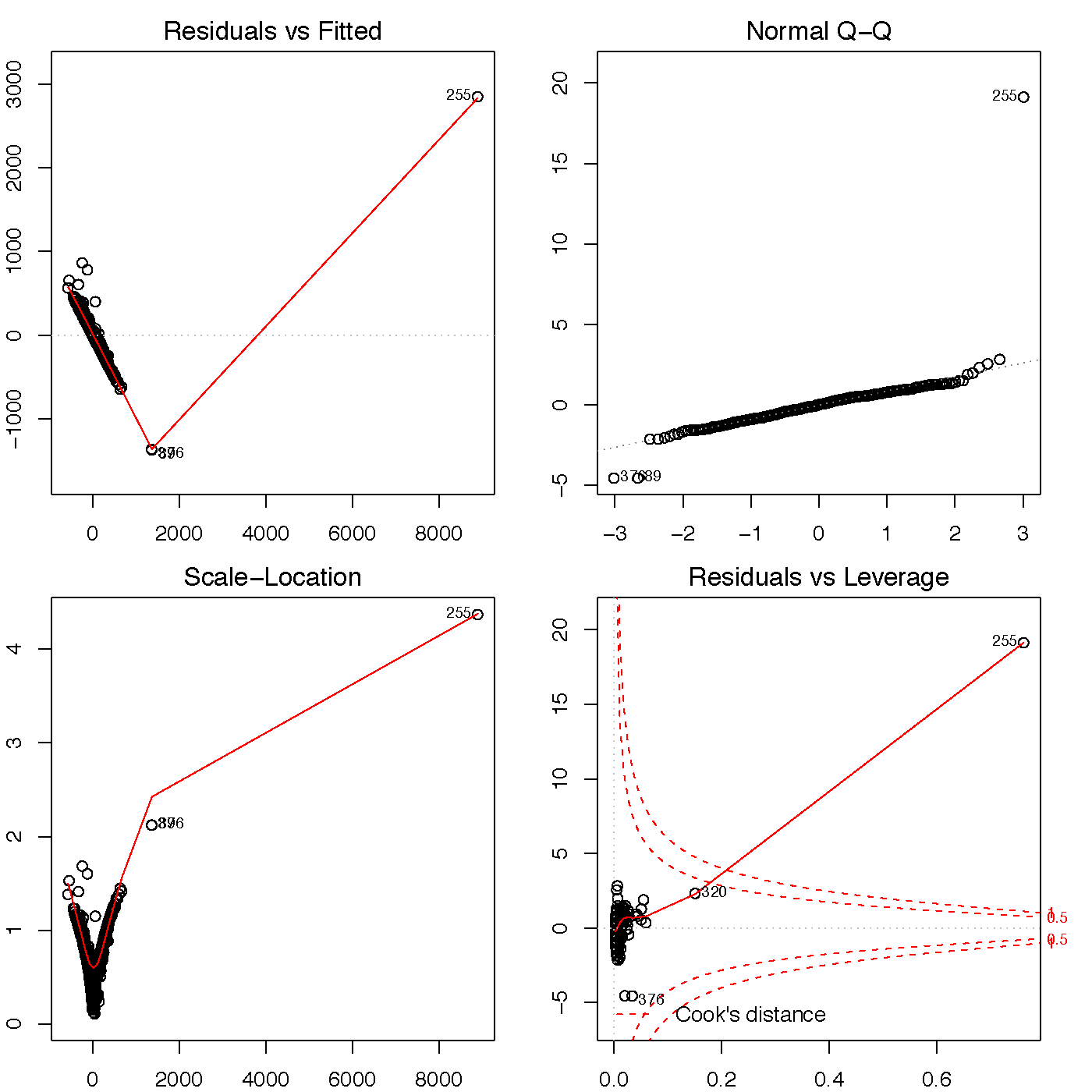
Looking at the four diagnostic plots in Figure 2 raises some concerns. The residuals vs fitted and scale-location maps each show a very clear pattern to the points, which indicates that this model hasn’t explained enough of the variance in our dependent variable. Except for one outlier, the points on the Q-Q plot stick pretty close to the fit line, so our data seems close to normal. The residuals vs leverage plot shows this same outlier outside the cook’s distance, which indicates that it could influence the regression fit. This outlier complicates the model, although it isn’t definitely an error, because of how heavily the drug activity in Kensington is clustered in a few very small areas.

Figure 3 is a map of the residuals from our linear model. We see a number of tracts in the higher classes, and some moderate clustering both south and north of Center City Philadelphia. This would tend to agree with the output in Figure 2 that we haven’t explained all of the variance in our model.

Geographically Weighted Regression

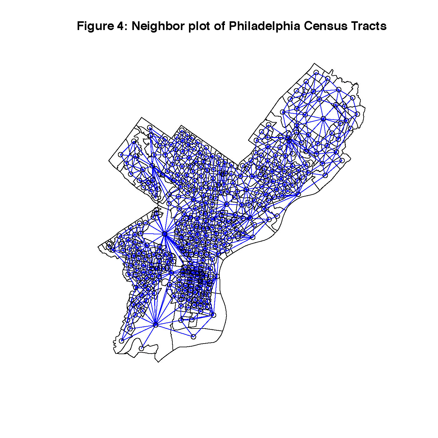
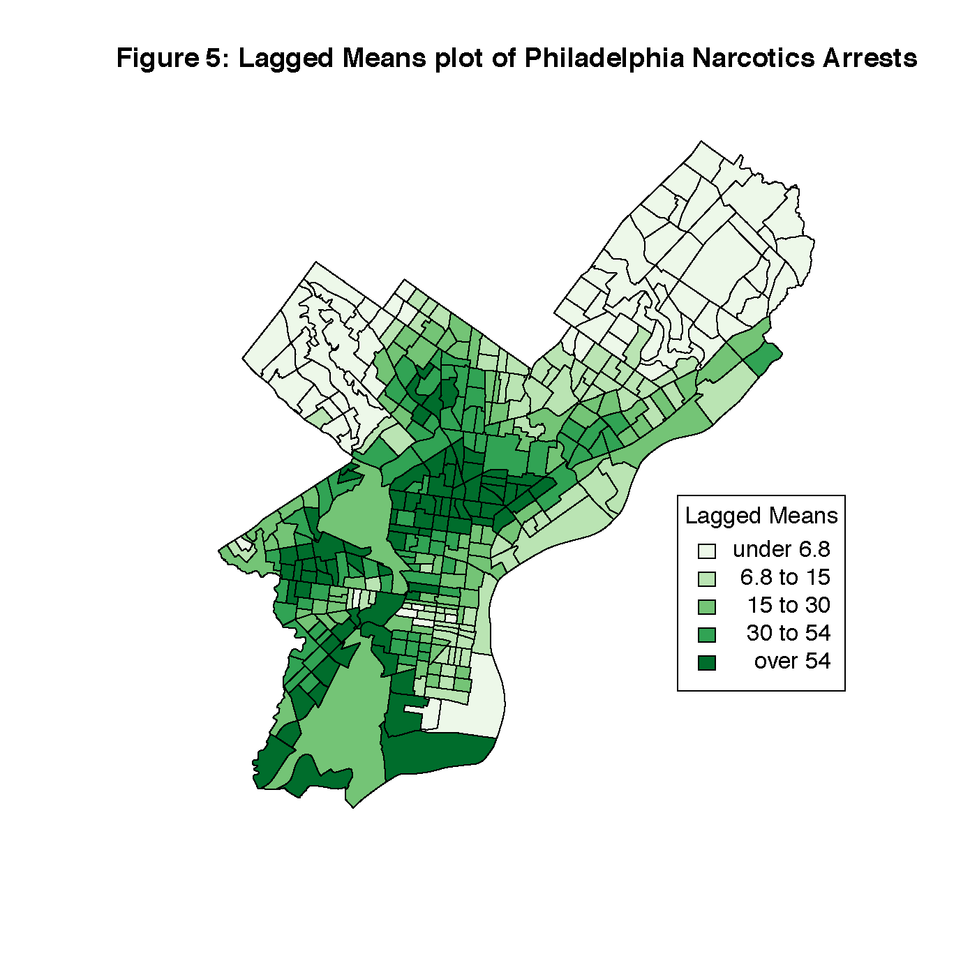
Figure 4 is a queen’s case map of the connections between census tracts in Philadelphia, and Figure 5 is the Lagged Means plot of the dependent variable. This shows us that there are two areas with very strong clustering of narcotics arrests, North Philadelphia/Kensington, and West Philadelphia. Both areas are adjacent to a busy subway and overhead railroad infrastructure that may serve to reduce eyes on the street.

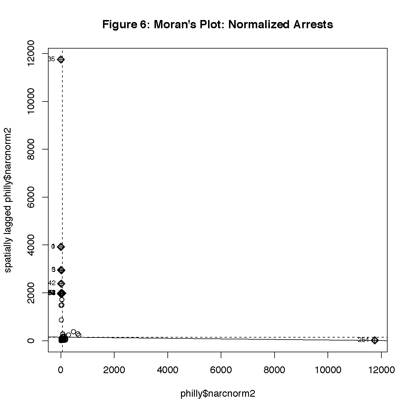
Figure 6 is a Moran’s plot. This plot is a little unusual. Most of the data is clustered close in the bottom left of the plot, and there is one data point far out in the bottom right corner. This causes the plot to zoom out far enough that looking for trends will not be very effective. To compare, Figure 7 is a Moran’s plot from the same data before normalization was applied, which is more readable. We see tight clustering of points in the bottom left, and a few other points loosely following the fit line to the top right. Seeing a pattern in this graph helps us confirm that our data is not all independent, and we may have some autocorrelation. The few outliers seen in Figure 6 could have been generated by data issues in the normalization process.

Out of a range of -.7 to 1.06, our Moran’s I statistic from the randomization test is -.012 with a p-value of .983. The Monte-Carlo simulation of Moran’s I gives us similar results, with a statistic of -.012 and a p-value of .996. Because these two calculations are not statistically significant, there is a chance that any apparent global correlation is a result of random chance and not meaningful for our study.

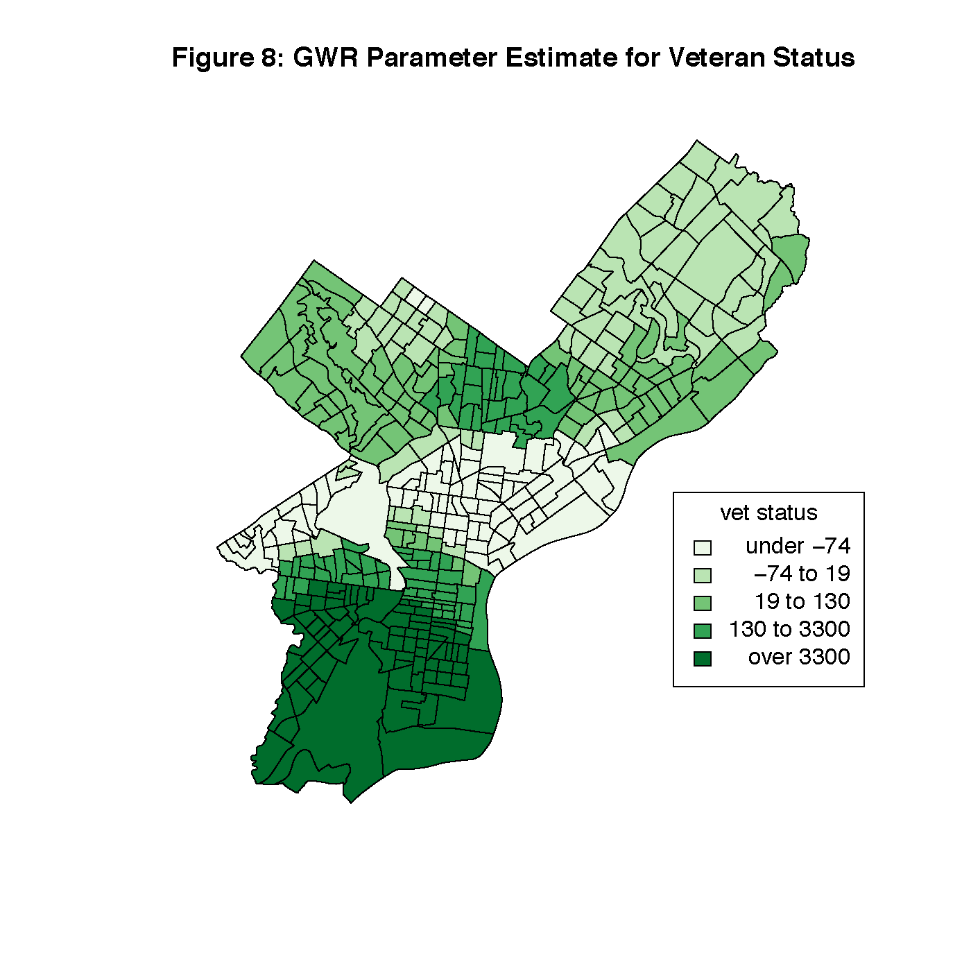
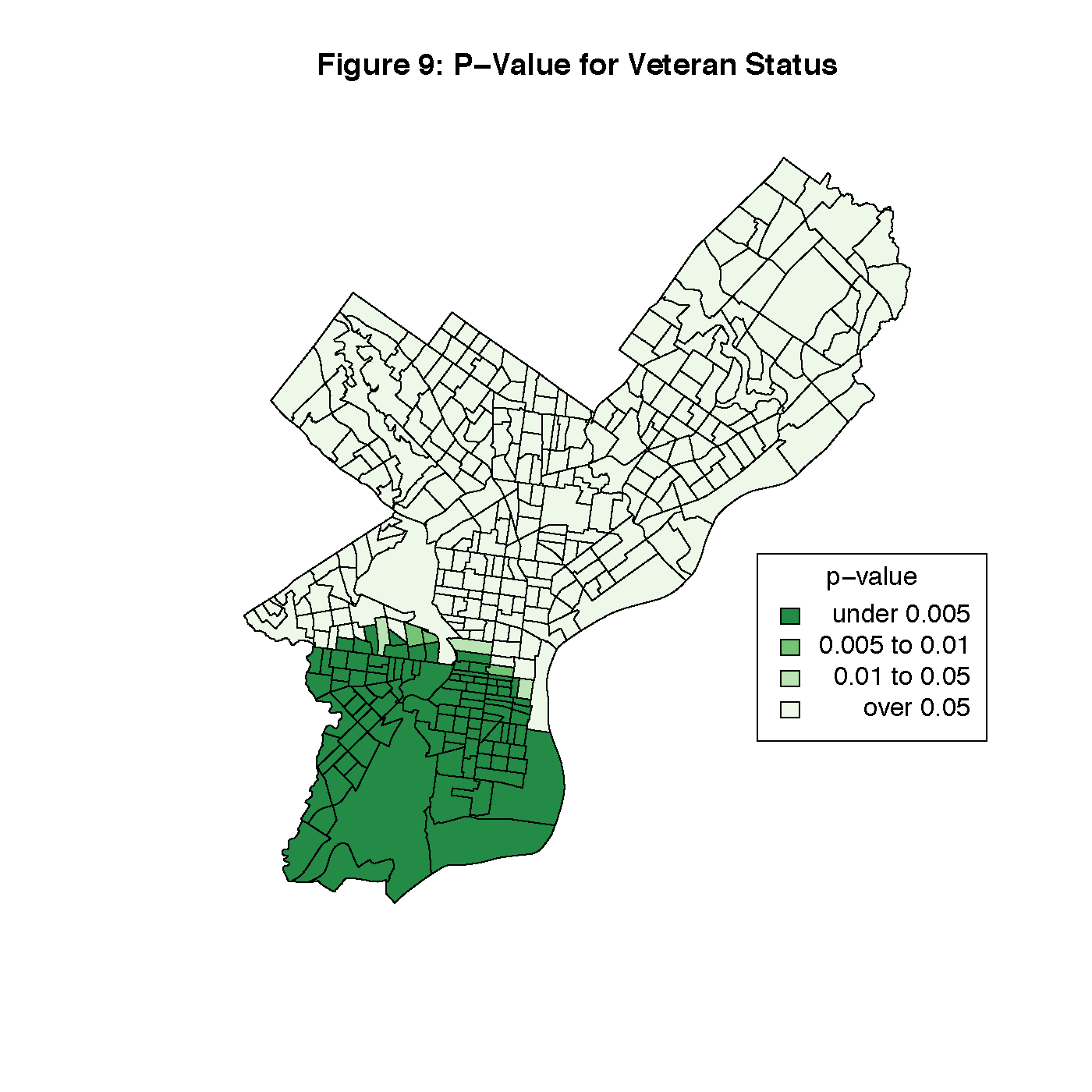
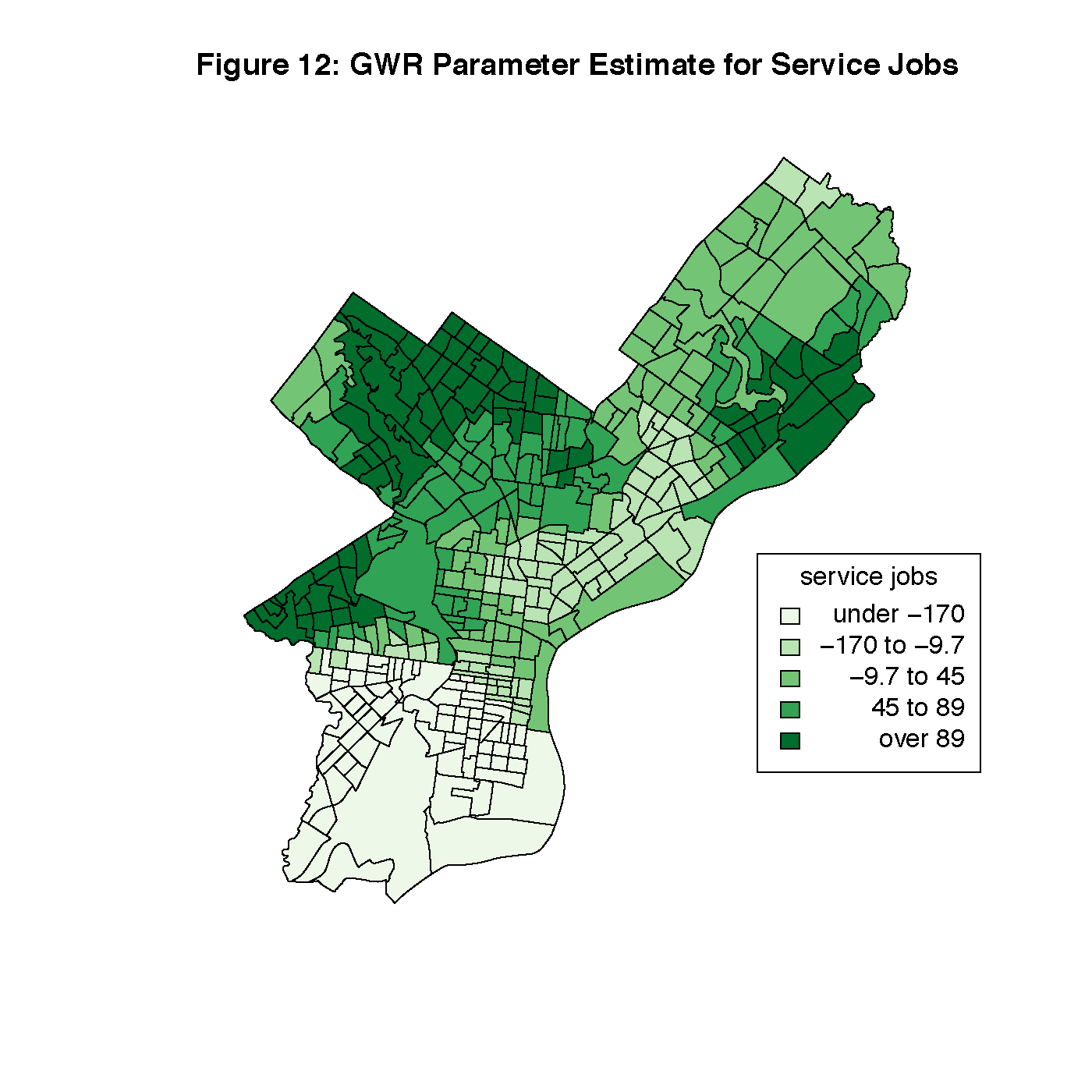
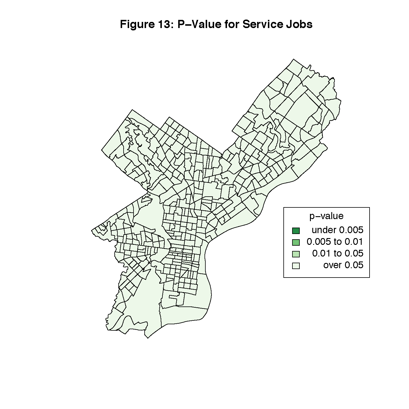
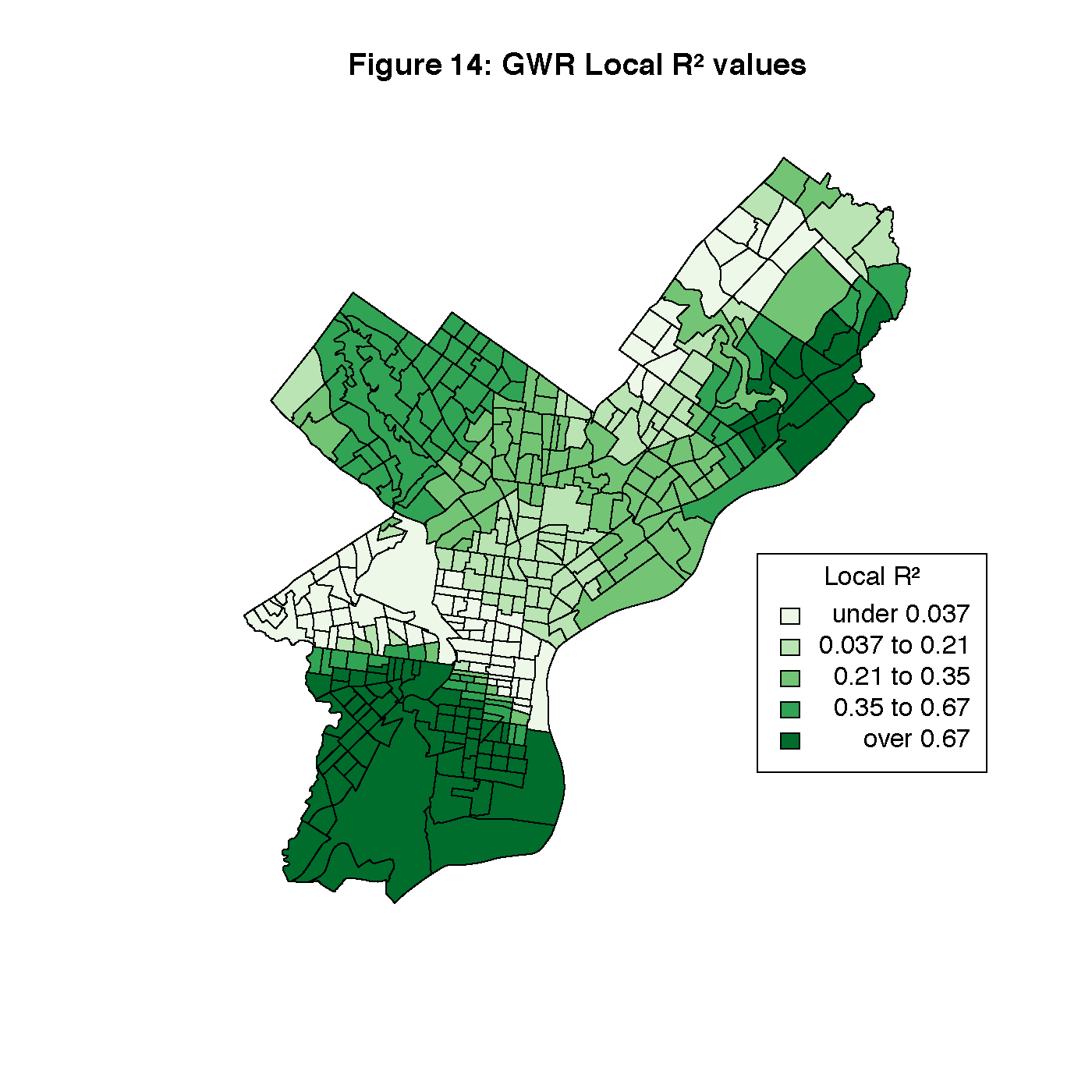
Figures 8 through 13 visualize the results of our Geographically Weighted Regression. Figures 11 and 13 are maps of the p-value for service jobs and per-capita income, both of which are not statistically significant through the whole map. Looking at Figures 8 and 9, we see that rate of veterans in the population is only statistically significant through the tracts in South Philadelphia, where the parameter estimate is the highest. However, Figure 14 is a map of the local R² values, and area with the highest values is that same portion of South Philadelphia, which would indicate that this variable may warrant closer investigation.

The data for this analysis was unexpected, and differs from our linear model quite a bit, but it demonstrates how important local analysis is for an issue like drug use that is so varied throughout the city.

Spatial Autoregression

The third model in this analysis was a Spatial Autoregressive model. Looking at this model, all three of our independent variables are still statistically significant, as they were with the linear model. The calculated value for rho is not statistically significant, which means we cannot reject the null hypothesis that there is no spatial autocorrelation. This is in line with the result the two Moran’s I calculations gave us. Looking at the AIC, the calculated value for the linear model is slightly lower than for this model, which tells us that this model does not give us much of an improvement over the linear model.

Call:lagsarlm(formula = philly$narcnorm2 ~ philly$vetnorm + philly$incomefix + 
    philly$servnorm, data = philly, listw = philly_neigh_lw)

Residuals:
       Min         1Q     Median         3Q        Max 
-1362.9837  -181.0117     9.8774   179.1920  2849.2338 
Type: lag 
Coefficients: (numerical Hessian approximate standard errors) 
                    Estimate  Std. Error z value  Pr(>|z|)
(Intercept)      -1.7925e+02  7.0600e+01 -2.5390  0.011117
philly$vetnorm    9.0798e+03  2.8015e+02 32.4106 < 2.2e-16
philly$incomefix -5.8178e-03  1.1931e-03 -4.8761 1.082e-06
philly$servnorm  -4.7740e+02  1.7280e+02 -2.7627  0.005732

Rho: 0.010573, LR test value: 0.25455, p-value: 0.61389
Approximate (numerical Hessian) standard error: 0.021215
    z-value: 0.49838, p-value: 0.61822
Wald statistic: 0.24838, p-value: 0.61822

Log likelihood: -2739.731 for lag model
ML residual variance (sigma squared): 92184, (sigma: 303.62)
Number of observations: 384 
Number of parameters estimated: 6 
AIC: 5491.5, (AIC for lm: 5489.7

Conclusion

The results received from these three models were mixed. The OLS and SAR regression models were statistically significant, though they indicated that there is more work to be done reducing the residuals. The results received from the GWR regression were a departure in that two of the variables were insignificant city-wide, and the third was called into question by very high R² values. Philadelphia’s drug problems seem to be pretty heavily clustered to specific neighborhoods, and the biggest takeaway from these results is that a citywide analysis might not be the most appropriate for this data. Another important point here is that an issue like this has many possible variables affecting it such as the built environment and police policies, so there is only so far an analysis based on demography can go.

Figures

Appendix: R code

rm(list = ls())

#load reqiured libraries
library(GISTools)
library(maptools)
library(spgwr)
library(spdep)
library(lm.beta)
library(pastecs)

#load data
philly <- readShapeSpatial("data/narc_join")
philly_acs <- read.csv("R11739357_SL140.csv")

#join CSV data to philly DF
philly@data <- data.frame(philly@data, philly_acs[match(philly@data[,"GEOID10"],philly_acs[,"Geo_FIPS"]),])

#SE_T083_001:    per capita income
#SE_T131_001 pop vet status 18 and over
#SE_T095_003 vacant houses

#SE_T033_006 unemployment pop over 16 - not used
#SE_T140_003 service job - not used
#SE_T145_002 no health insurance coverage - not significant
#SE_T098_001 median year structure built - unused

#normalize the count of narcotics incidents
philly$popinthousands <- philly$SE_T001_001 / 1000
philly$narcnorm2 <- philly$Count_ / philly$popinthousands
#unemployment
philly$unempnorm <- philly$SE_T033_006 / philly$SE_T033_001
#veteran
philly$vetnorm <- philly$SE_T131_002  / philly$SE_T131_001
#vacant houses
philly$vacantnorm <- philly$SE_T095_003 / philly$SE_T095_001
#service jobs
philly$servnorm <- philly$SE_T140_003 / philly$SE_T140_001
  #remove bad values from data created by 0 population tracts
na.inf <- function (x) {
  x[is.infinite(x)] <- 0
  return(x)
}
na.zero <- function (x) {
  x[is.na(x)] <- 0
  return(x)
}

philly$narcnorm2 <- na.zero(philly$narcnorm2)
philly$unempnorm <- na.zero(philly$unempnorm)
philly$vetnorm <- na.zero(philly$vetnorm)
philly$vacantnorm <- na.zero(philly$vacantnorm)
philly$servnorm <- na.zero(philly$servnorm)
philly$incomefix <- na.zero(philly$SE_T083_001)
philly$narcnorm2 <- na.inf(philly$narcnorm2)
philly$unempnorm <- na.inf(philly$unempnorm)
philly$vetnorm <- na.inf(philly$vetnorm)
philly$vacantnorm <- na.inf(philly$vacantnorm)
philly$servnorm <- na.inf(philly$servnorm)


vals <- cbind(philly$narcnorm2, philly$vetnorm, philly$incomefix, philly$servnorm)
stat.desc(vals)
summary(vals)

pdf(file = "f1.narcoticsarrestschoropleth.pdf")
narcnorm.shades <- auto.shading(philly$narcnorm2, cols=brewer.pal(5,"Greens"))
choropleth(philly, philly$narcnorm2, shading = narcnorm.shades)
title("Figure 1: Narcotics Arrests, 2012-2016")
choro.legend(2725857,238144, narcnorm.shades, title = "arrests per thousand")
dev.off()

#create our linear model
# lm01 <- lm(philly$Count_ ~ philly$SE_T033_001)
# lm02 <- lm(philly$Count_ ~ philly$SE_T033_001 + philly$SE_T083_001)
# lm03 <- lm(philly$narcnorm2 ~ philly$SE_T033_001 + philly$SE_T083_001 + philly$SE_T131_001 + philly$SE_T095_003 + philly$SE_T140_003)
#lm04 <- lm(philly$narcnorm2 ~  philly$vetnorm + philly$incomefix + philly$vacantnorm )
lm04 <- lm(philly$narcnorm2 ~  philly$vetnorm + philly$incomefix + philly$servnorm )
summary(lm04)
#add standardized betas
lm04.std <- lm.beta(lm04)
summary(lm04.std)
#dianostic plots for lm04
pdf(file = "f2.lm04diag.pdf")
par(mar=c(2,2,2,2),mfrow=c(2,2))
plot(lm04)
par(mfrow=c(1,1))
dev.off()

#lm04 residuals
lm04residshades = auto.shading(lm04$residuals, cols=brewer.pal(5,"Greens"))
pdf(file = "f3.lm04residchoropleth.pdf")
choropleth(philly, lm04$residuals, shading = lm04residshades)
title("Figure 3: Residuals from linear model lm04")
choro.legend(2729559,251723.8, lm04residshades, title = "residuals")
dev.off()

#create neighbor list and plot
philly_neighbors <- poly2nb(philly)
pdf(file = "f4.neighbormap.pdf")
plot(philly, main = "Figure 4: Neighbor plot of Philadelphia Census Tracts")
plot(philly_neighbors, coordinates(philly), add=T, col='blue')
dev.off()

#create lagged means
philly_neigh_lw <- nb2listw(philly_neighbors)
narclag <- lag.listw(philly_neigh_lw, philly$narcnorm2)
#create lagged means plot
laggedmeanshades = auto.shading(narclag, cols=brewer.pal(5,"Greens"))
pdf(file = "f5.laggedmeanchoropleth.pdf")
choropleth(philly, narclag, shading =laggedmeanshades)
title("Figure 5: Lagged Means plot of Philadelphia Narcotics Arrests")
choro.legend(2729559,251723.8, laggedmeanshades, title = "Lagged Means")
dev.off()

#Moran's I
moran.range <- function(lw) {
  wmat <- listw2mat(lw)
  return(range(eigen((wmat + t(wmat))/2)$values))
}
moran.range(philly_neigh_lw)
#approximate test statistic using normal distribution
moran.test(philly$narcnorm2, philly_neigh_lw)
#calculate the test statistic using 10,000 random trials
moran.mc(philly$narcnorm2, philly_neigh_lw, 10000)
#Moran's Plot
pdf(file = "f6.moransplotnorm.pdf")
moran.plot(philly$narcnorm2, philly_neigh_lw)
title("Figure 6: Moran's Plot: Normalized Arrests")
dev.off()
pdf(file = "f7.moransplotraw.pdf")
moran.plot(philly$Count_, philly_neigh_lw)
title("Figure 7: Moran's Plot: Raw Arrest Count")
dev.off()

#GWR
philly.bw <- gwr.sel(philly$narcnorm2 ~ philly$vetnorm + philly$incomefix + philly$servnorm, data = philly, gweight = gwr.Gauss)
philly.gwr <- gwr(philly$narcnorm2 ~ philly$vetnorm + philly$incomefix + philly$servnorm, data = philly, bandwidth = philly.bw, gweight = gwr.Gauss, hatmatrix = T)
gwr.df <- slot(philly.gwr$SDF, "data")

summary(philly.gwr)
names(philly.gwr)
names(philly.gwr$SDF)
print(philly.gwr)
anova(philly.gwr)

#calculate the t-score and p value
gwr.df$vet_tval <- gwr.df$philly.vetnorm / gwr.df$philly.vetnorm_se
gwr.df$vet_pval <-pt(gwr.df$vet_tval, 380, lower.tail = FALSE)
gwr.df$income_tval <- gwr.df$philly.incomefix / gwr.df$philly.incomefix_se
gwr.df$income_pval <- pt(gwr.df$income_tval, 380, lower.tail = FALSE)
gwr.df$serv_tval <- gwr.df$philly.servnorm / gwr.df$philly.servnorm_se
gwr.df$serv_pval <- pt(gwr.df$serv_tval, 380, lower.tail = FALSE)

pdf(file = "f8.vetparamchoropleth.pdf")
vetparamshades = auto.shading(gwr.df$philly.vetnorm, cols=brewer.pal(5,"Greens"))
choropleth(philly, gwr.df$philly.vetnorm, shading=vetparamshades)
title("Figure 8: GWR Parameter Estimate for Veteran Status")
choro.legend(2729559,251723.8, vetparamshades, title = "vet status")
dev.off()

pdf(file = "f9.vetpvalchoro.pdf")
vetpvalshades <- shading(c(0.005, 0.01, 0.05), cols = rev(brewer.pal(4, "Greens")))
choropleth(philly, gwr.df$vet_pval, shading = vetpvalshades)
title("Figure 9: P-Value for Veteran Status")
choro.legend(2729559,251723.8, vetpvalshades, title = "p-value")
dev.off()

pdf(file = "f10.incomeparamchoropleth.pdf")
par(mar=c(1,1,2,1))
incomeparamshades = auto.shading(gwr.df$philly.incomefix, cols=brewer.pal(5,"Greens"))
choropleth(philly, gwr.df$philly.incomefix, shading=incomeparamshades)
title("Figure 10: GWR Parameter Estimate for Per Capita Income")
choro.legend(2711398,241846.7, incomeparamshades, title = "per cap income")
dev.off()

pdf(file = "f11.incomepvalchoro.pdf")
incomepvalshades <- shading(c(0.005, 0.01, 0.05), cols = rev(brewer.pal(4, "Greens")))
choropleth(philly, gwr.df$income_pval, shading = incomepvalshades)
title("Figure 11: P-Value for Per Capita Income")
choro.legend(2729559,251723.8, incomepvalshades, title = "p-value")
dev.off()

pdf(file = "f12.servparamchoropleth.pdf")
servparamshades = auto.shading(gwr.df$philly.servnorm, cols=brewer.pal(5,"Greens"))
choropleth(philly, gwr.df$philly.servnorm, shading=servparamshades)
title("Figure 12: GWR Parameter Estimate for Service Jobs")
choro.legend(2729559,251723.8, servparamshades, title = "service jobs")
dev.off()

pdf(file = "f13.servpvalchoro.pdf")
servpvalshades <- shading(c(0.005, 0.01, 0.05), cols = rev(brewer.pal(4, "Greens")))
choropleth(philly, gwr.df$serv_pval, shading=servpvalshades)
title("Figure 13: P-Value for Service Jobs")
choro.legend(2729559,251723.8, servpvalshades, title = "p-value")
dev.off()

#R^2
pdf(file = "f14.localr2.pdf")
localr2shades = auto.shading(gwr.df$localR2, cols=brewer.pal(5,"Greens"))
choropleth(philly, gwr.df$localR2, shading=localr2shades)
title("Figure 14: GWR Local R² values")
choro.legend(2729559,251723.8, localr2shades, title = "Local R²")
dev.off()

#Spatial Autoregressive Models
lm04.lag <- lagsarlm(philly$narcnorm2 ~ philly$vetnorm + philly$incomefix + philly$servnorm, data = philly, philly_neigh_lw)
summary(lm04.lag)
anova(lm04.lag, lm04)